Part A
1.0
In this part, I accepted the terms and conditions of using the model from HuggingFace, specifically the DeepFloyd/IF-I-XL-v1.0 diffusion models, and grabbed a HuggingFace token from my account.
Then I was able to pull the model using the starter code provided, pulling both Stage I and Stage II of the DeepFloyd diffusion model. Afterwards, I used the precomputed text embeddings. Using the precomputed textual embeddings, I was able to get the following nice images.
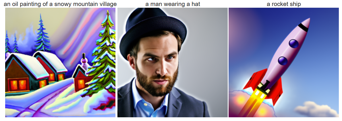
Generated images using precomputed textual embeddings.
We see that the pretrained diffusion models work!
1.1
In this step, I took a clean image of the Campanile which is provided as a sample image, and iteratively added noise to it based on a predetermined forward pass equation. The idea is that t indicates the number of timesteps, or in this case, like the number of layers of a noising neural network. If t is big, then that means that the original image is passing through a greater number of layers in a noising neural network. Specifically, I used the alphas_cumprod variable at all the different timesteps, denoted as alpha_t, using the following equation:
Using the equation, I was able to noise the image X_t, following a standard Gaussian distribution with mean of

Original Image of the Campanile
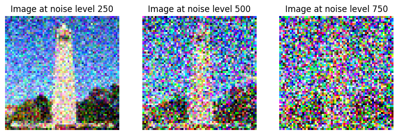
Noised Image of the Campanile at varying timesteps (values of t)
Through this, the image was denoised. We can see that, based on what was given by the starter code, alpha_t's value went smaller and smaller as t grew, which means that less and less of the original image x_0 contributed to the final image when compared to the Gaussian noise. This will naturally lead to the image being noisier, which is the observed result.
1.2
Given a noisy image that we have just managed to create with layers of iterative noising operations, we now try to denoise the image
For my first method, I attempt to use Gaussian Blur as a denoising strategy. Since noise is typically higher frequency, by blurring we preserve only lower frequencies, and thereby this is an effective approach at removing the noise in an image.
Obviously this has some drawbacks, most notably that this method also destroys high-frequency information from the image itself, but this is our first attempt.
We try to denoise the image for each of the resulting noised images for the three different noise levels (values of t) from the previous part. Here are our results.
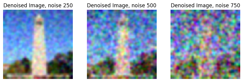
Denoised Images of the Campanile at varying noise levels (values of t)
Clearly, this is a mess and Gaussian Blur does not work so well.
1.3
Now we try to use some sort of neural network model to (intelligently) denoise. We shall take advantage of something called a UNet, which is basically something that takes in something and returns something else, of the same shape. The special part of this UNet is that its hidden layer is much smaller than both the input and output shape, and it tends to be like a funnel, each successive hidden layer from the input reducing the hidden layer dimensions until the smallest dimension hidden layer is reached, then inverting the funnel and increasing the hidden layer size every time. We use the stage_1.unet, which is pretrained on samples of x0 and xt (i.e. original as input, noised as output). We use it to recover (expected) Gaussian noise for a good image by passing in the original image and getting the expected noised image, then taking their difference. With this noise, however, we have to do more processing, as we have to then multiply this noise by
, then subtract the clean image from the noised image, as this method respects our original forward pass.
Running the forward passes on a set of images, we have the following result:
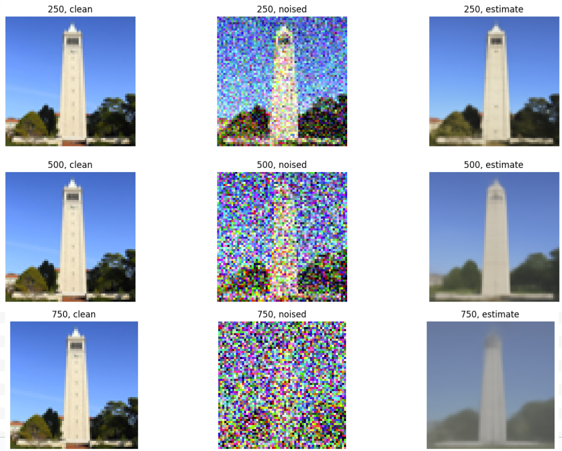
Denoised Images of the Campanile at varying noise levels (values of t) with One Step Denoising, compared to Original and the Noised Image
With this, we conclude the One-Step solution is clearly more effective than the Gaussian Denoising solution.
1.4
Can we do better, even though the last part could achieve good results?
Here, we take advantage of diffusion model's nature, which is that they are supposed to be used to denoise in an iterative process
Since our forward pass took T=1000 steps, we should (in theory) also take this many steps in denoising. But we can skip steps for the sake of minimzation of inference latency.
We instead use strided timesteps, and our iteratively denoised equation should be written as follows

Cited Berkeley
To test this model, I noise the test Campanile image to nearly the max, at t=990, and attempt to iteratively denoise. I use a stride of 30, and output my result every 5 strides. Here are my results.

Strided Image, Noised Results
Clearly the rightmost image has been the most noisy, and has gotten much better as the solution iteratively denoises the noisy image.
The final denoised result with iterative denoising of a t=990 noised image of the campanile is as follows:
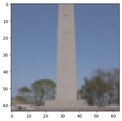
Result of Iterative Denoising
Here is result of One Step Denoising of the same image:
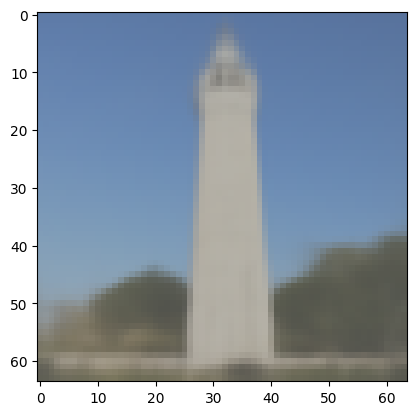
Result of One Step Denoising
Here is result of Gaussian Denoising of the same image:
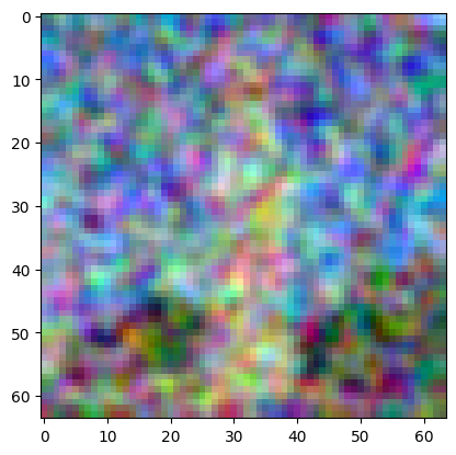
Result of Gaussian Denoising
Now seen side by side, all of them put together

Comparison of All Denoising Types and Categories
1.5
Since we can denoise very very noised images, what if we pass in images of pure random noise to the iterative denoiser?
We can, and using the same text embeddings for the unet as for the last question (the text embedding for "a high quality image"), we get the following results:
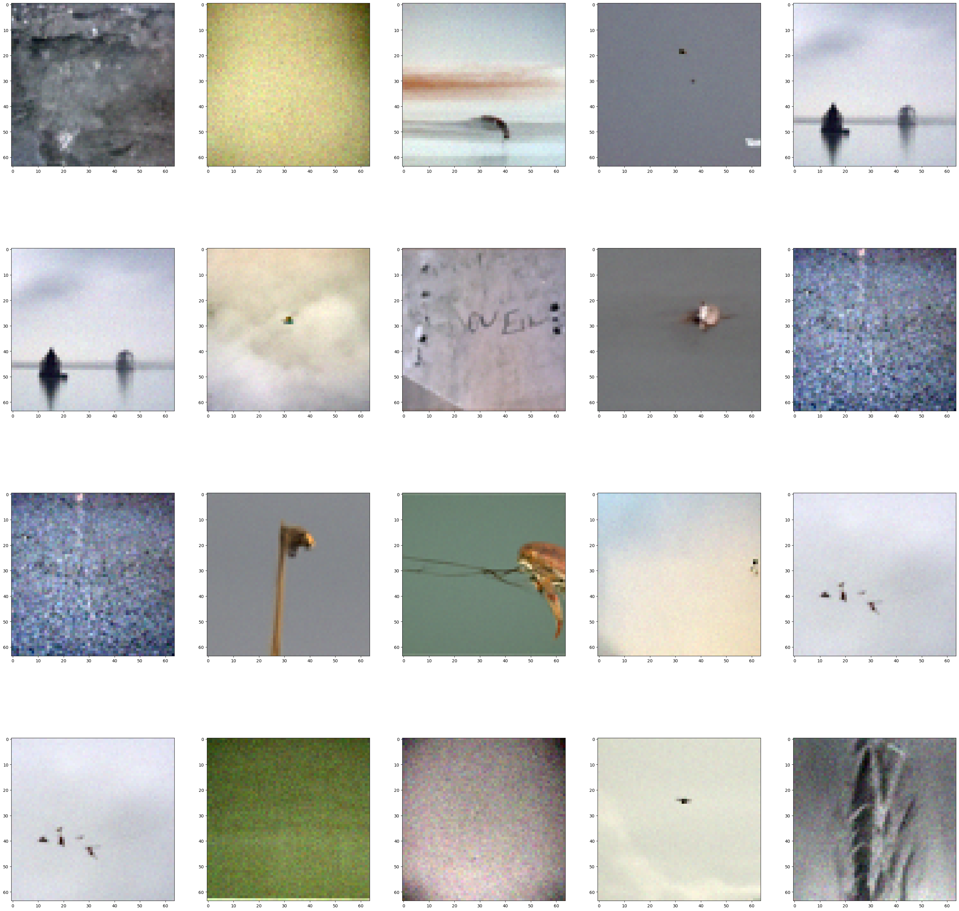
Newly Generated Images
We see all these look somewhat real, but they can clearly look better.
1.6
To get better results, we essentially try to make it look more "real". The way we do this is kind of like inspiration from Project 3, where we create the extrapolation from the mean. The idea is basically that we want to have a conditional and unconditional noise estimate (noise estimate of conditional prompt and noise estimate of unconditional prompt, i.e. noise estimate of u-net when you pass into it a text embedding representing a null string). Then, we extrapolate the image towards the conditional estimate by factor of gamma.
With this extrapolation, we can get images that lean closer to the side of the image that we want to generate, based on our text embedding, than previously.
Here are our results (gamma=7):
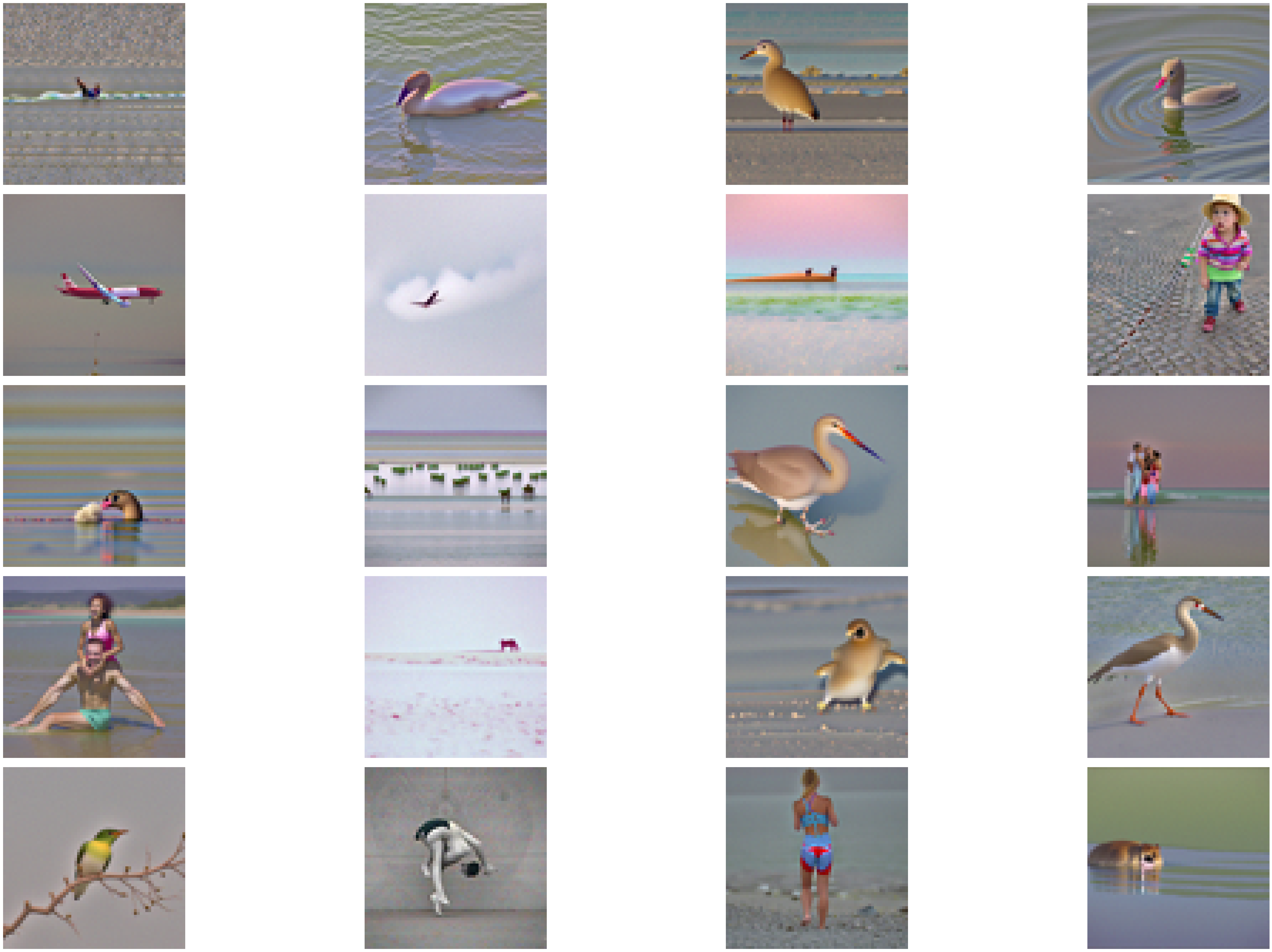
Extrapolated (Better) Generated Images
The results are much better!
1.7
Now lets play more with this iterative denoising model. We want it to generate cooler things!
Suppose we noise an image and we have the model regenerate a denoised image. Since this model is doing the extrapolation thing with gamma=7, we can expect very creative results, and very good looking results. But do these good looking results (i.e creative results) match what we initially put in, the real result?
We vary the noise level to manipulate our results. The noise level indicates the distance from pure noise the starting image is. 1 indicates a greater amount for noise that we could add to the image, as it indicates an image that is much closer to pure noise than an image represented by a larger noise level. We vary the noise level from 1 to 10.
Showing a subset of the results I generated, we have:
1: Original Test
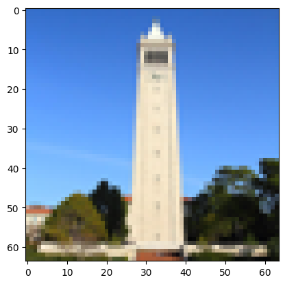
Original
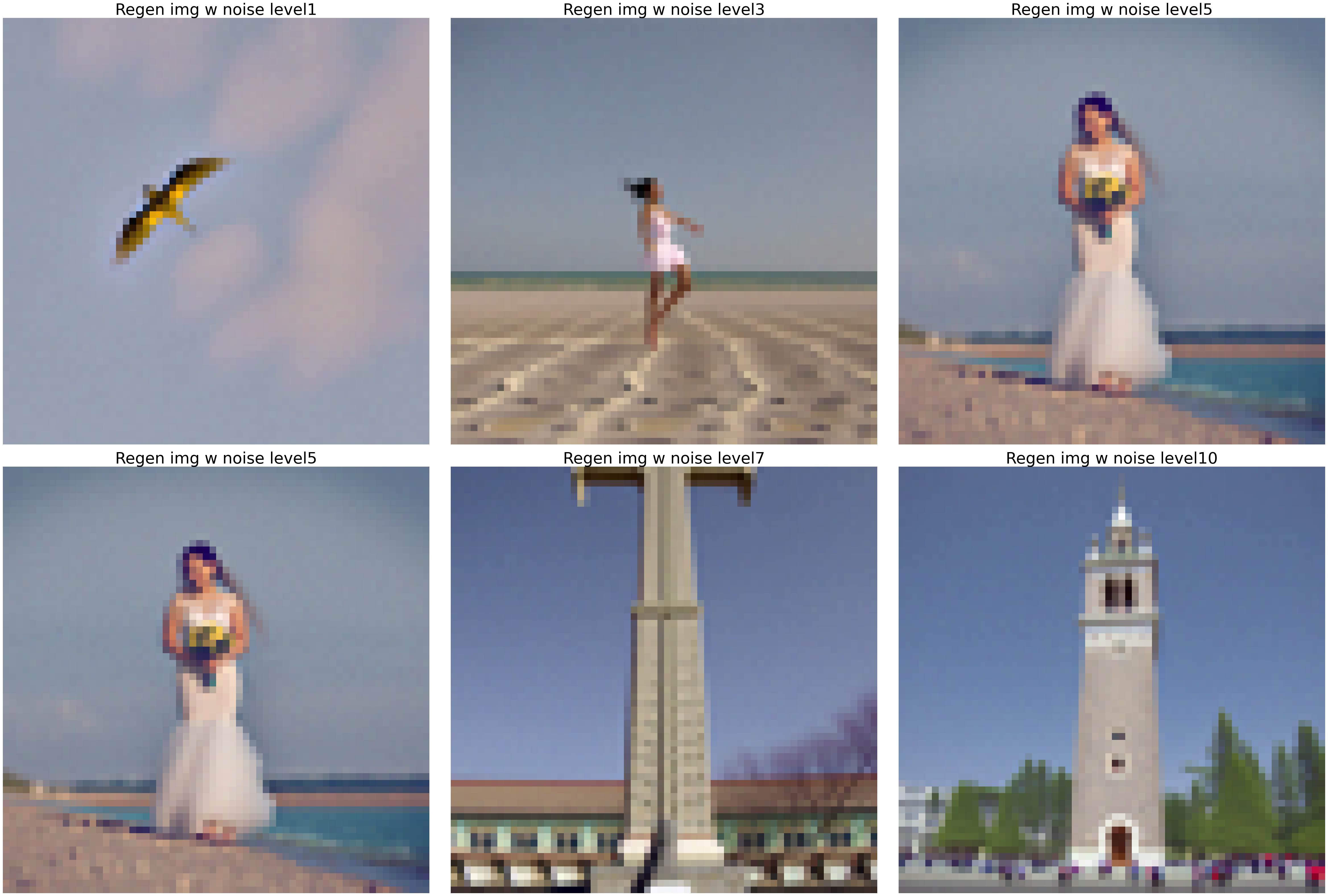
Campanile Edited Image
2: Berkeley Tree
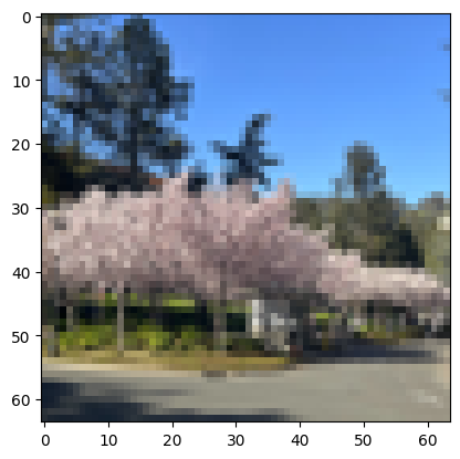
Original
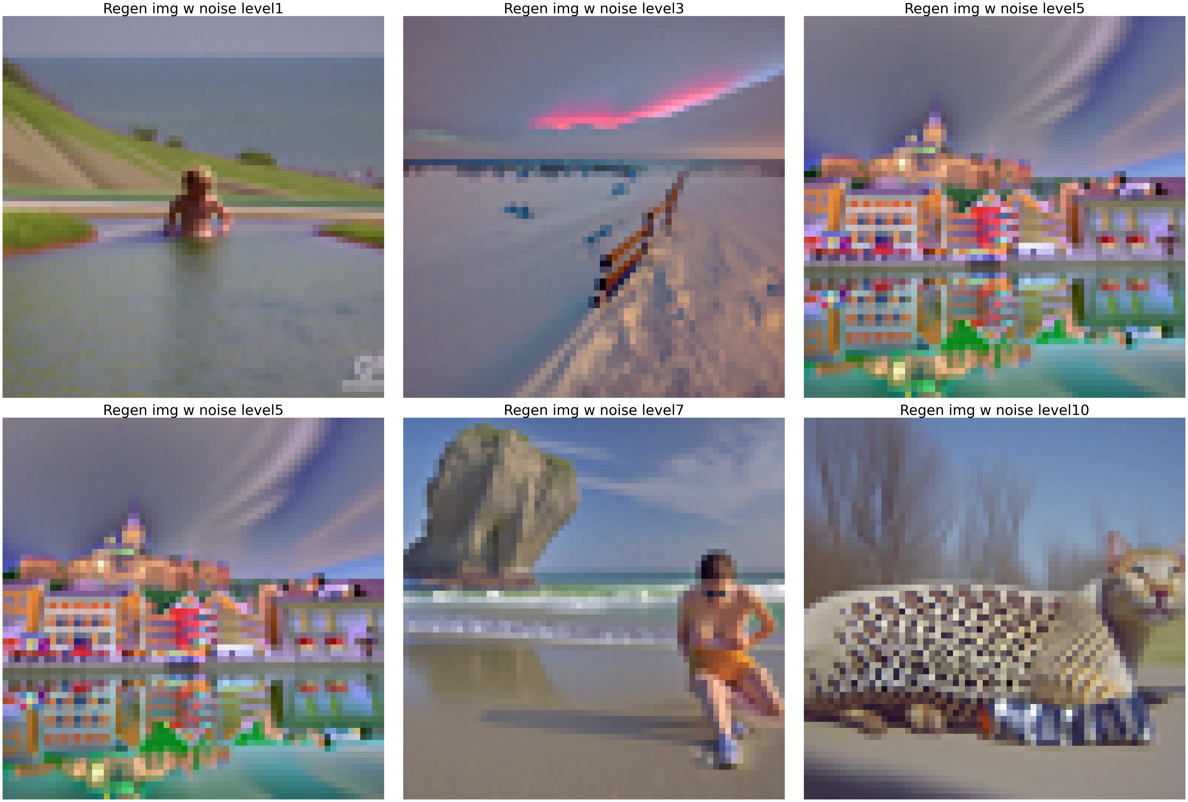
Berkeley Tree Edited Image
3: Cottage Monterey
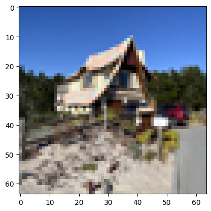
Original
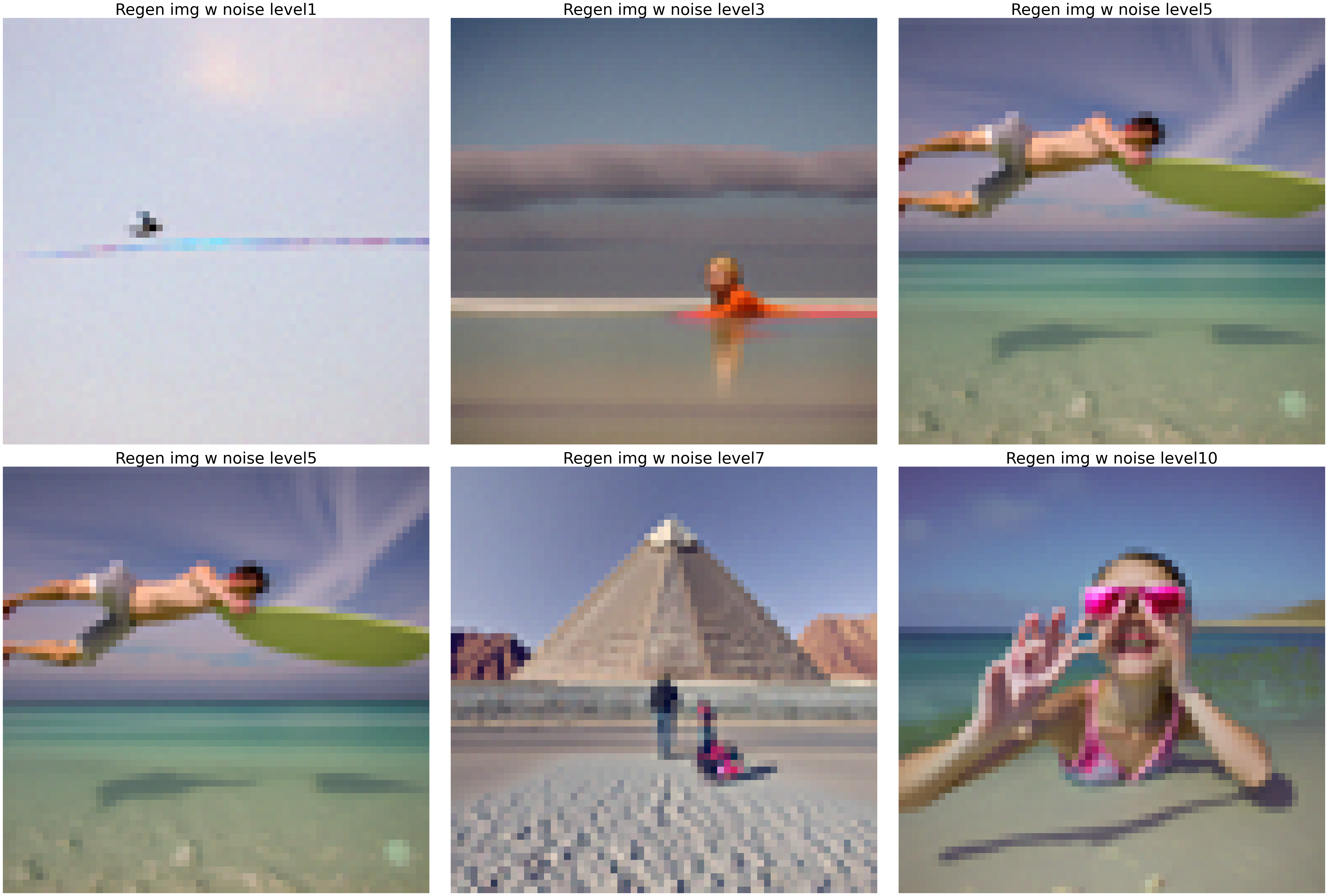
Cottage Monterey Edited Image
Wow! The denoising completely changed the image!
1.7.1
Now we do the same thing for handdrawn / clipart / cartoon images.
1: Random Avocado

Original

Avocado Edited Image
2: Cartoon Car

Original

Cartoon Car Edited Image
3: Handdrawn Image 1

Original

First Handdrawn Edited Image
4: Handdrawn Image 2

Original

Second Handdrawn Edited Image
5: Handdrawn Image 3

Original

Third Handdrawn Edited Image
1.7.2
Could we now try to only change a segment of the image, i.e., have the diffusion model only selectively edit the image? Perhaps only the head of a person in an image, or only the tip of a tower? Lets try.
We make a mask of pixels (1 somewhere, 0 elsewhere) and have the mask be the same shape as the image. Then, using an equation, we force x_t to have the same values as the original, at pixels where the mask equals 0.
where f is the forward pass.
Our results are as follows:
Original Campanile
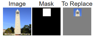
Original, Mask, Replaced Section

Impainted Original Image
Hat Person
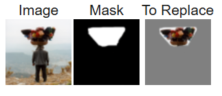
Original, Mask, Replaced Section

Impainted Person Image
UCSD Library
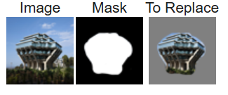
Original, Mask, Replaced Section

Impainted Person Image
1.7.3
Now we shall attempt to guide the image generation process to something interesting, rather than just "a high quality photo".
Prompt: "a rocket ship" with original test image

Rocket Ship Campanile
Prompt: "a rocket ship" with Stanford Hoover Tower

Rocket Ship Hoover
Prompt: "a rocket ship" with Random Tree

Rocket Ship Tree
Prompt: "a rocket ship" with Hospital

Rocket Ship Hospital
Prompt: "a rocket ship" with Church

Rocket Ship Church
Prompt: "a rocket ship" with Canton Tower

Rocket Ship Canton Tower
Prompt: "a rocket ship" with HK skyline

Rocket Ship HK
1.8
Here, we will be creating visual anagrams, images that look one way when looked from a certain angle (for example, right side up), and a different way when flipped.
In order to do this, we must obtain two noise results based on the two desired outcomes, and average the noises to get the final desired noise.
Our noise algorithm is as follows:
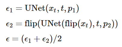
Anagram Algorithm
Where flip is flipping the image 180 degrees across an axis (here the horizontal one).
We create anagrams for the case of "A visual anagram where on one orientation "an oil painting of people around a campfire" is displayed and, when flipped, "an oil painting of an old man" is displayed." Here is the results:
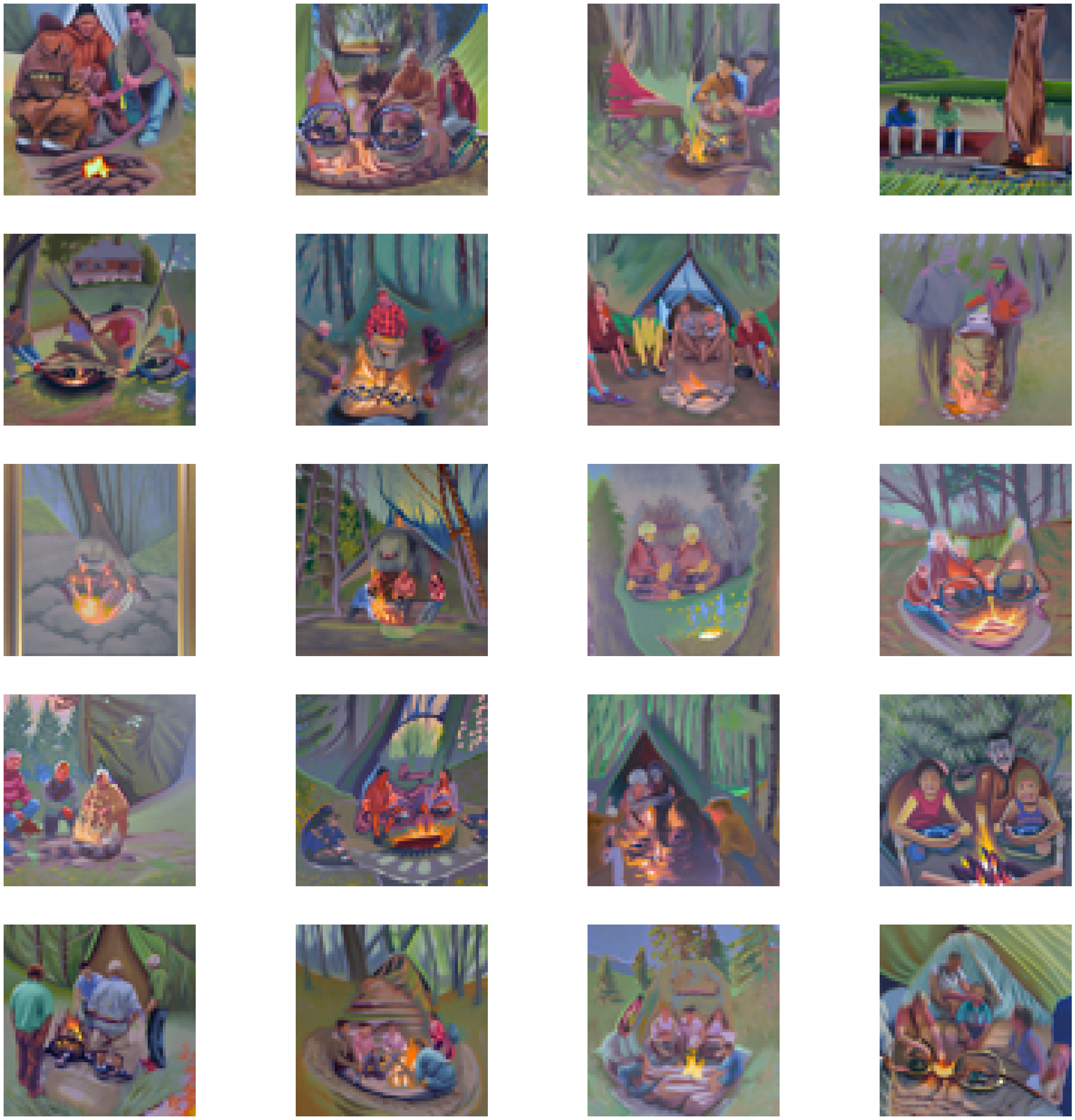
People around campfire + Old Man
Now for "a pencil" when normally seen and "a rocket ship" when flipped
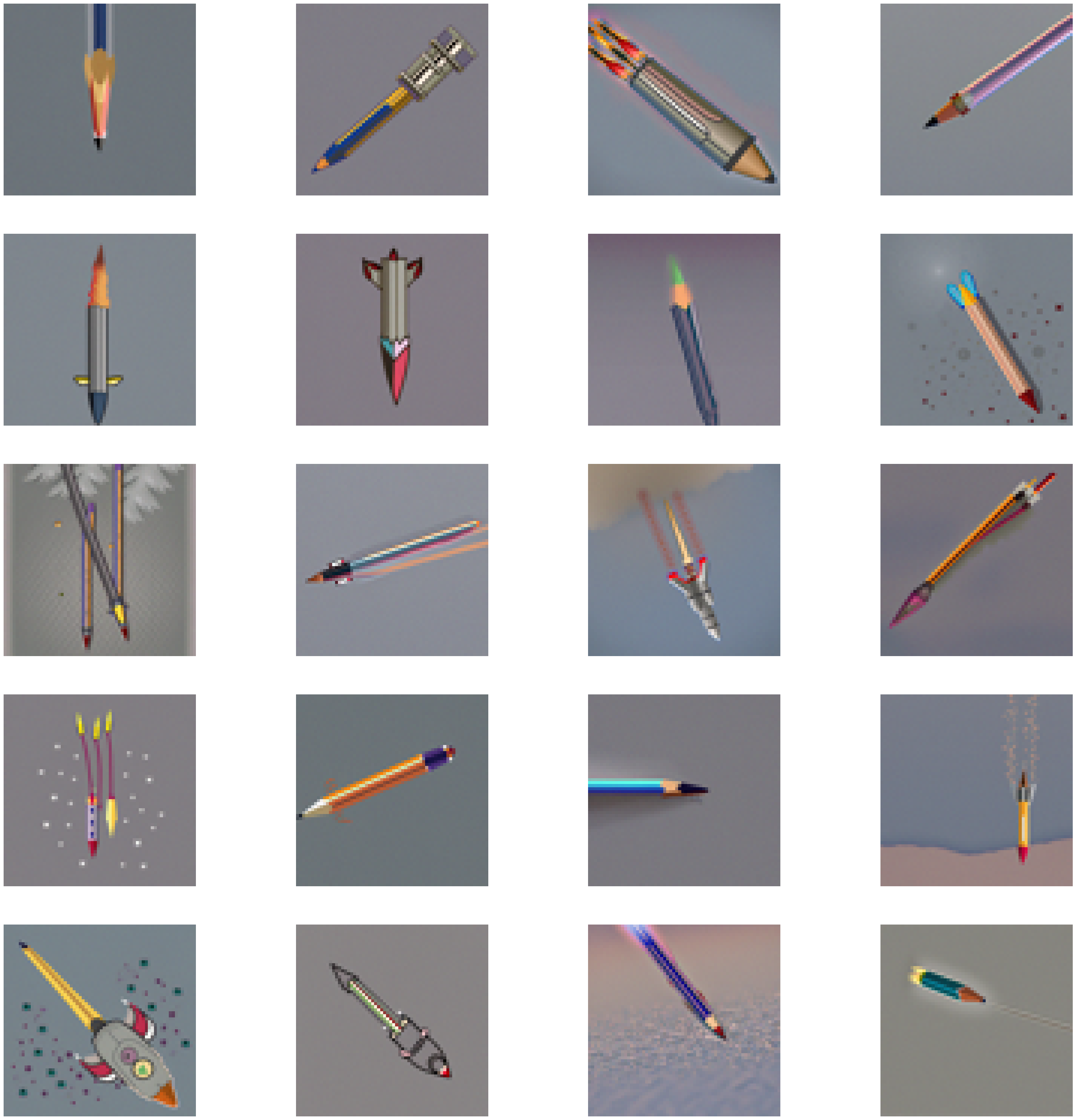
Pencil + Rocket
Now, "a photo of a hipster barista" when normally seen and "a photo of a dog" when flipped
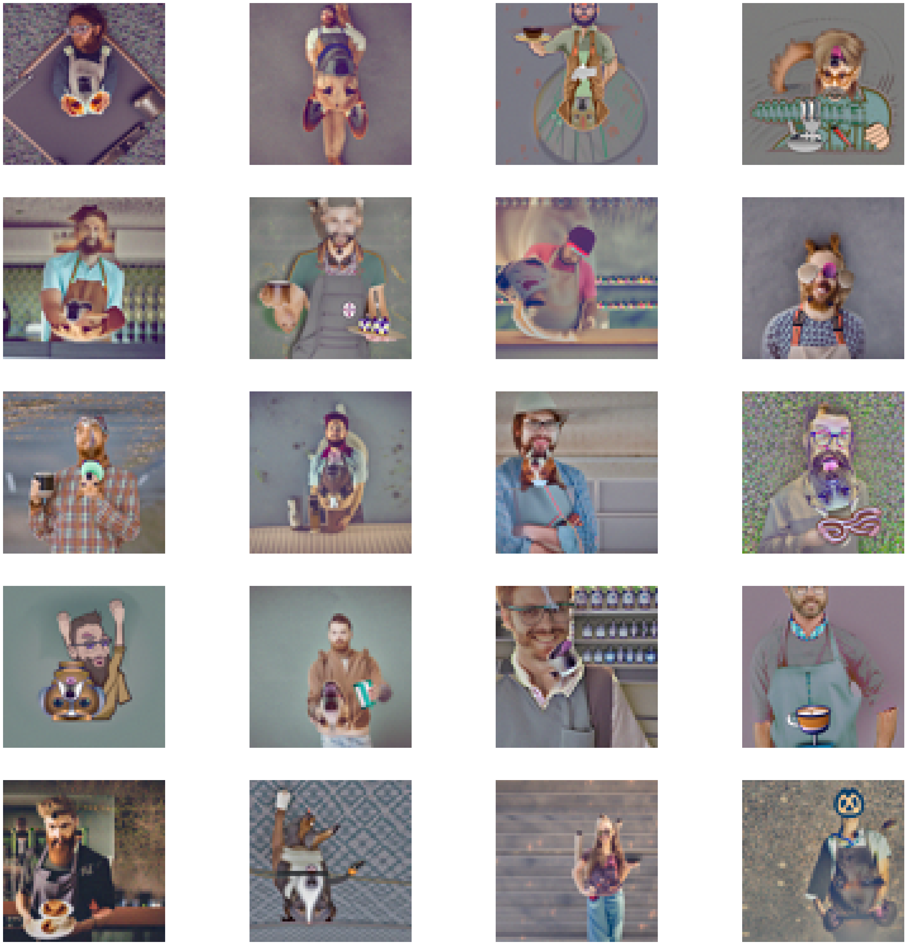
Hipster Barista + Dog
1.9
Now we will do the final step of this project, which is to create hybrid images, images that look one way when seen from close, and another way when seen from afar.
In order to do this, we must take the two noises that are generated from the differing text embedding prompts, and pass one of them through a high pass filter and the other through a low pass filter. Then, we set the final noise to the sum of these two noises.
Here are our results:
"Lithography of waterfalls" when far away and "Lithography of skull" when close
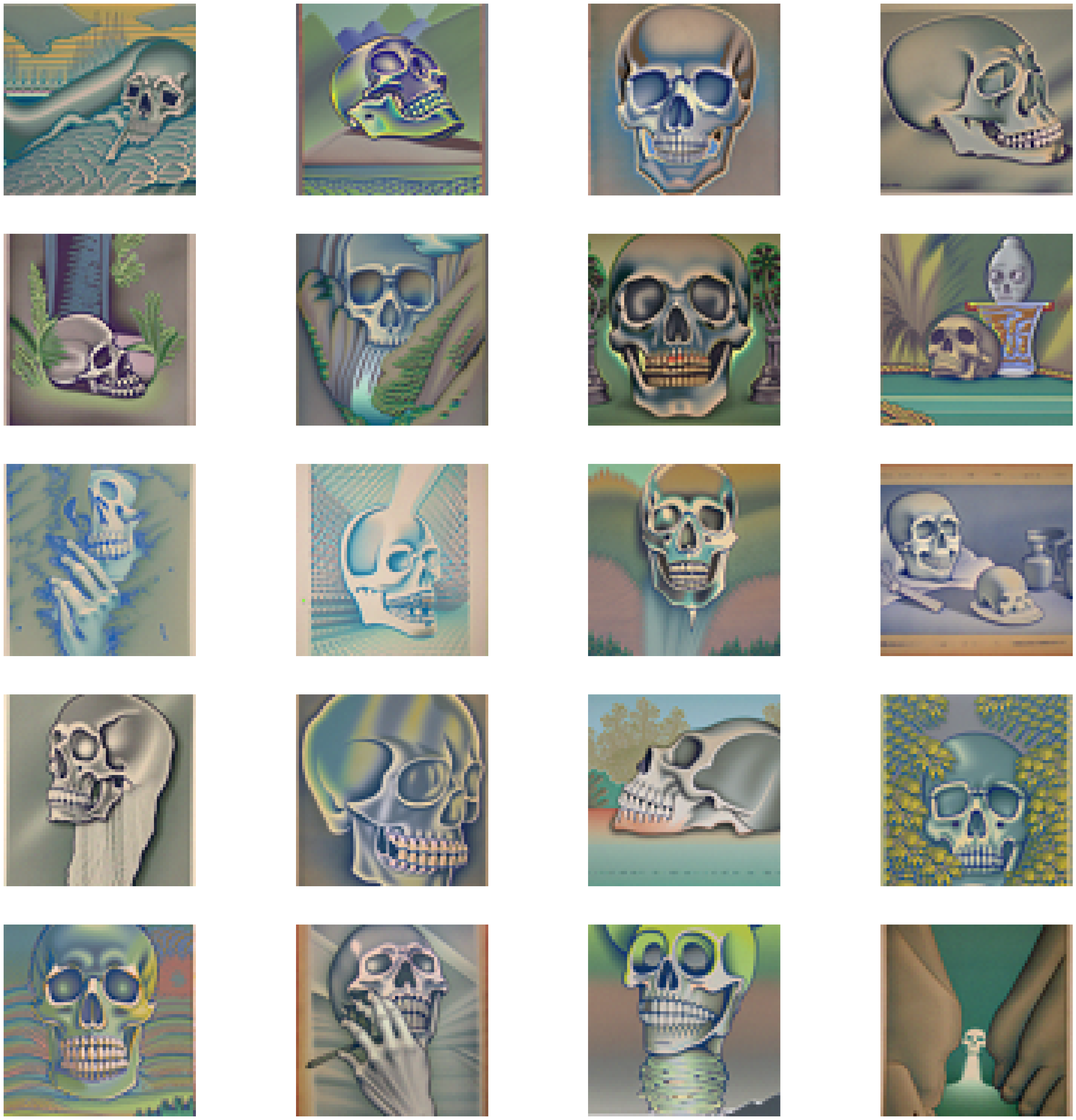
Waterfall + Skull
"People around campfire" when far away and "Snowy Mountain Village" when close
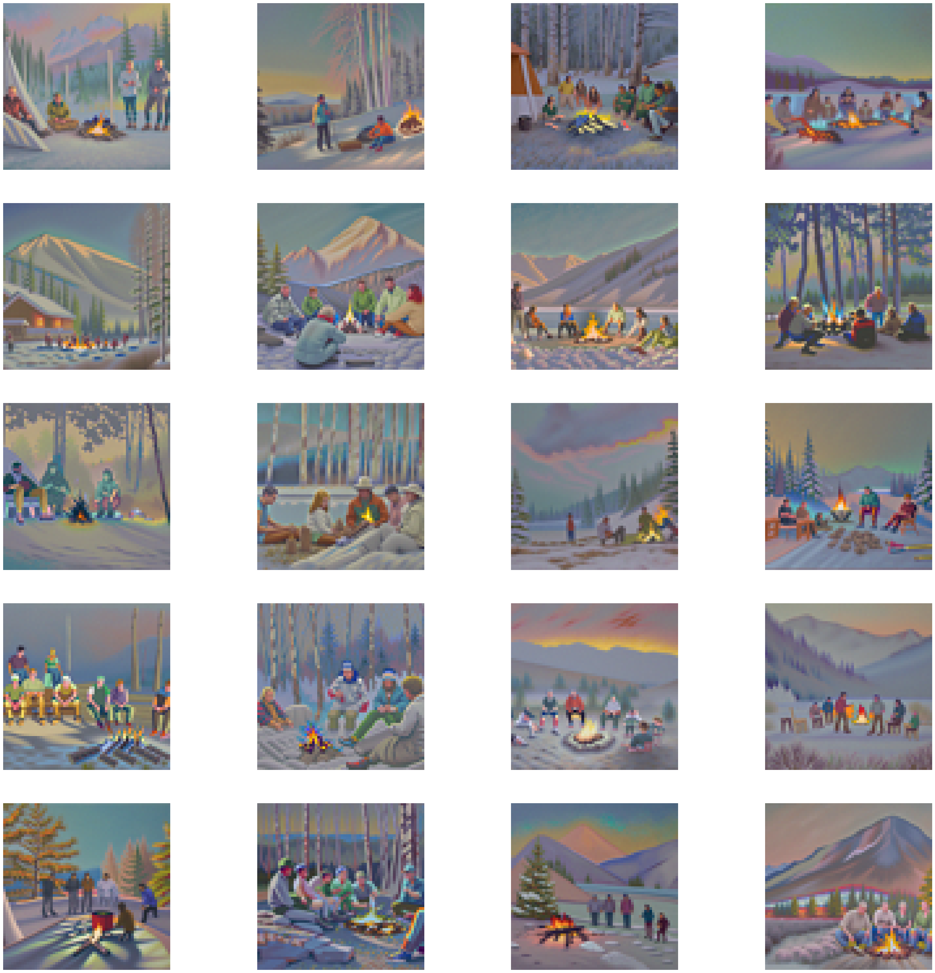
People around campfire + Snowy mountain village
"Rocket ship" when far away and "Man wearing a hat" when close
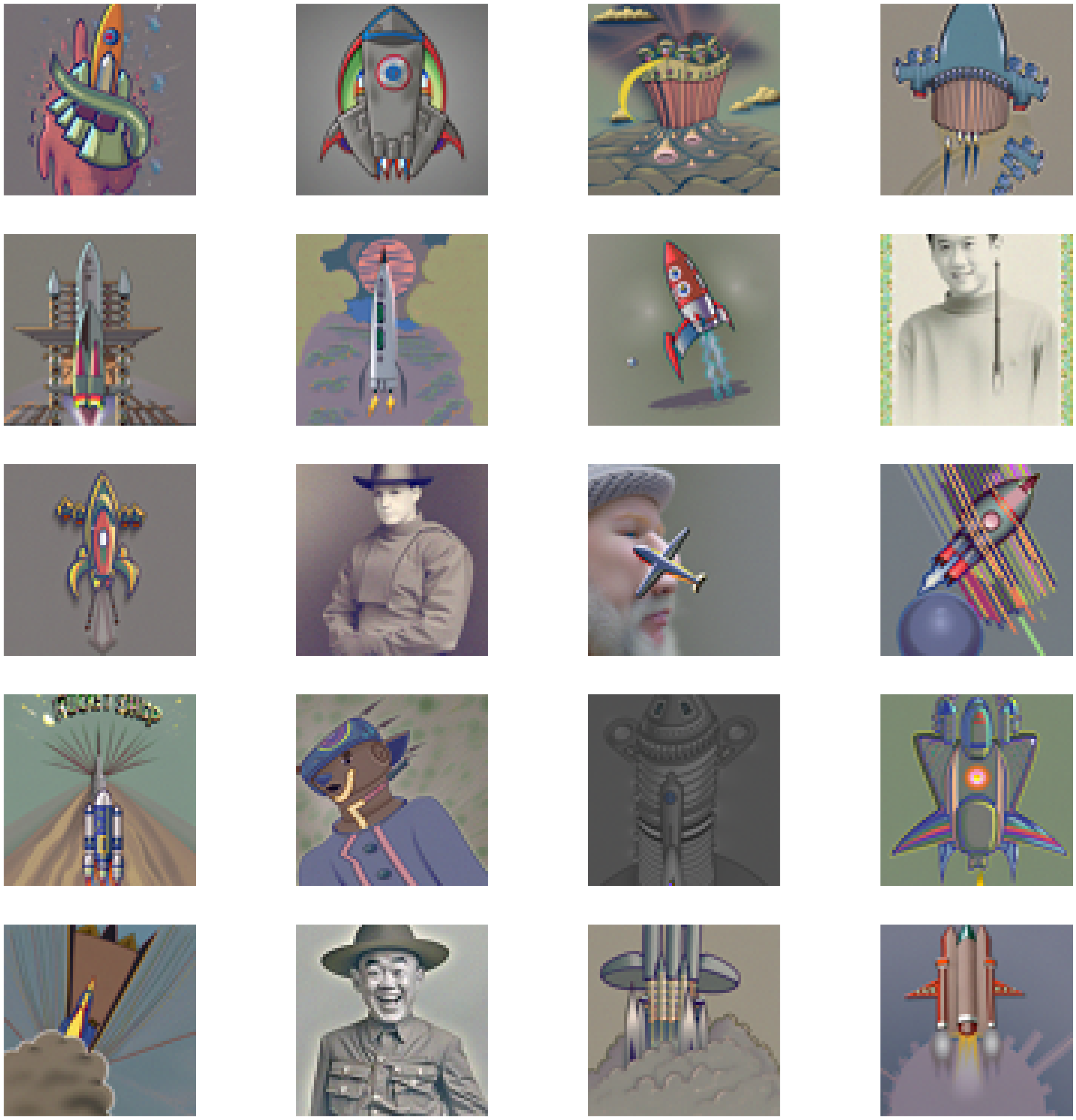
Hat Man + Rocket ship
We can see the last result is a little bit weird. I believe this is because the task is very challenging to generate, and the (pretrained) model is perhaps not powerful enough to generate good results for Hat Man and Rocket Ship.
Part B
Such cool results from Part A! However, in Part A, we have only been using other people's diffusion models? How do they work, and can we build our own diffusion model! In this section I will be building my own diffusion models, which will serve the noble purpose of denoising images, as well as generating them! What fun!
1
1.1
To start off the second part of the project, we have to build a UNet, and this Unet should be shaped exactly how the one we used from Part A is shaped. It should have same dimensions for input and output, and a hidden dimension within the UNet which contains a more compact representation of the information that is passed in the input. The reason for this compactness is that we hope the denoiser can get a sort of compact representation of core properties of the noised image from the information represented in the initial image. So, the part of the model from the input to this compact representation can be thought of as a projection of the (noisy) input image down to a compact representation, and the latter part (compact -> output), can be thought of as reconstruction of an image from the compact representation.
The structure of the UNet Model is as follows:
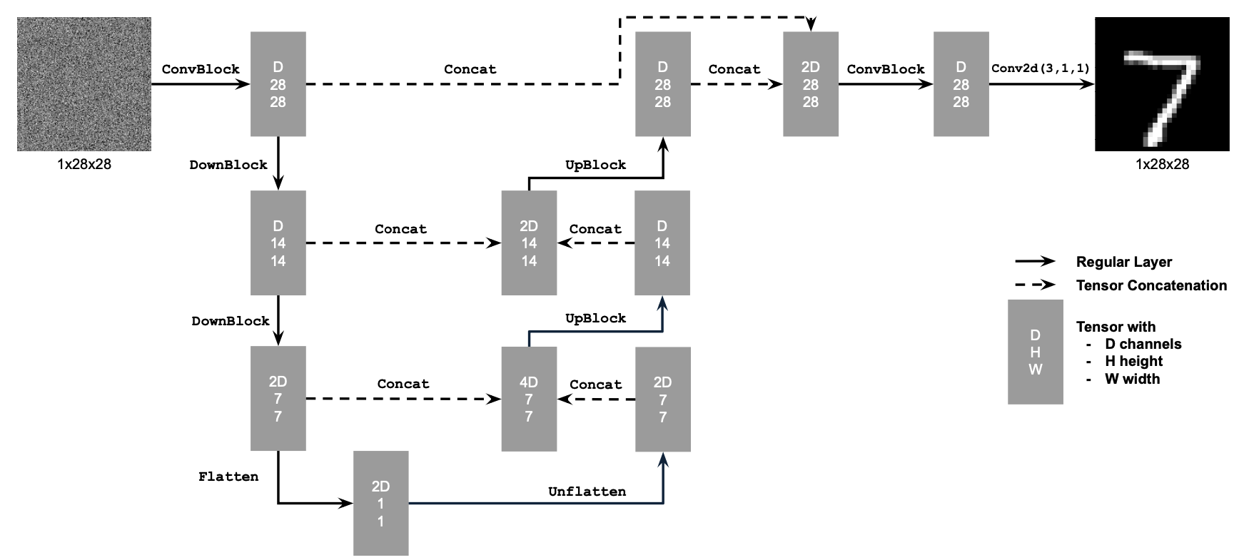
Architecture for basic UNet
Here is what each atomic model substructure represents:
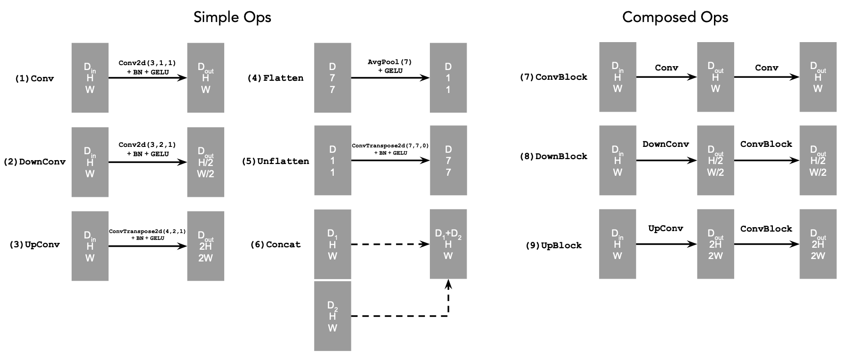
Atomic Architecture
Here, D consists of the hidden dimension, and the more compact representation is derived from the fact that the image is shrunk to a latent representation of 1x1 from 28x28. The size of D kind of determines the number of nodes of information that we want to keep track of.
1.2
Here, our goal is to successfully implement a noising scheme for the clean image, which we import from torchvision.datasets.MNIST. Using our noising scheme, we then will have data to train our denoiser. This data naturally will be (input, output) pairs of noised and clean versions of the same image
With this data, we define a hyperparameter sigma which is the fraction of noise we include in the image, acting as a coefficient of the standard gaussian noise. We vary sigma (coefficient of Gaussian noise) from an array ranging from 0-1.
Noised Images with respect to Sigma looks like this:
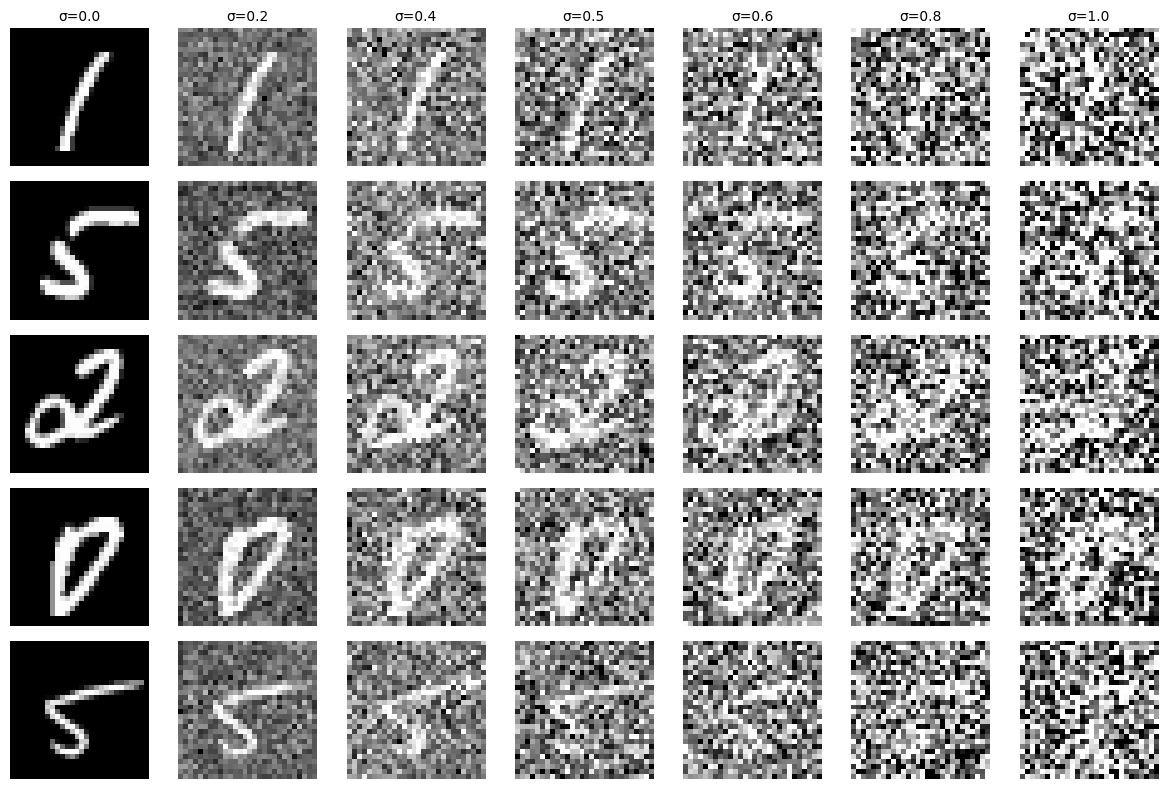
Noised Images over Different Sigma
The loss we will optimize over is:
where D_theta is the denoising model, and z is the noised image we will pass in as input.
1.2.1
Now we train the UNet model!
We train using the architecture described above! Here, we exclusively use images noised with sigma = 0.5. We use a batch size of 256, and an Adam optimizer system of 1e-4. Our hidden dimension of the UNet, D, we set it to be 128, allowing our diffusion model to capture ample features from the input image.
With the course staff's recommendation, we train the diffusion model over 5 epochs and plot the average loss over each step (i.e. each batch). Here is our Log Loss varied over the steps.
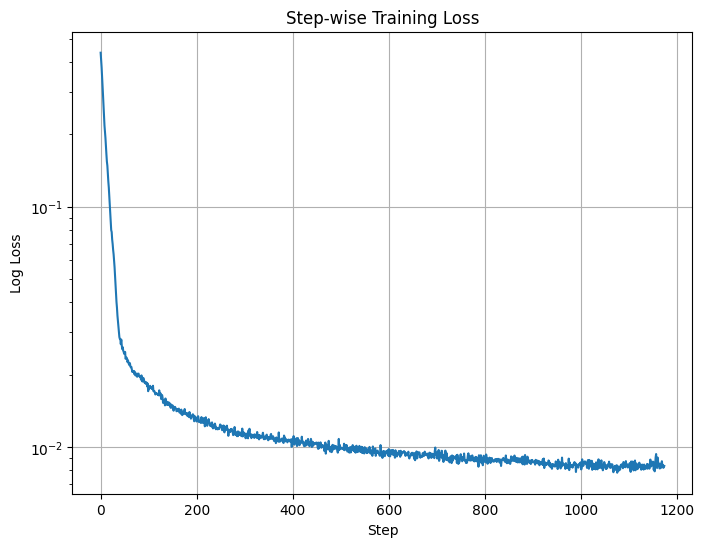
Log Loss over Steps for Unconditional UNet
Below is the results of training over 1 epoch!
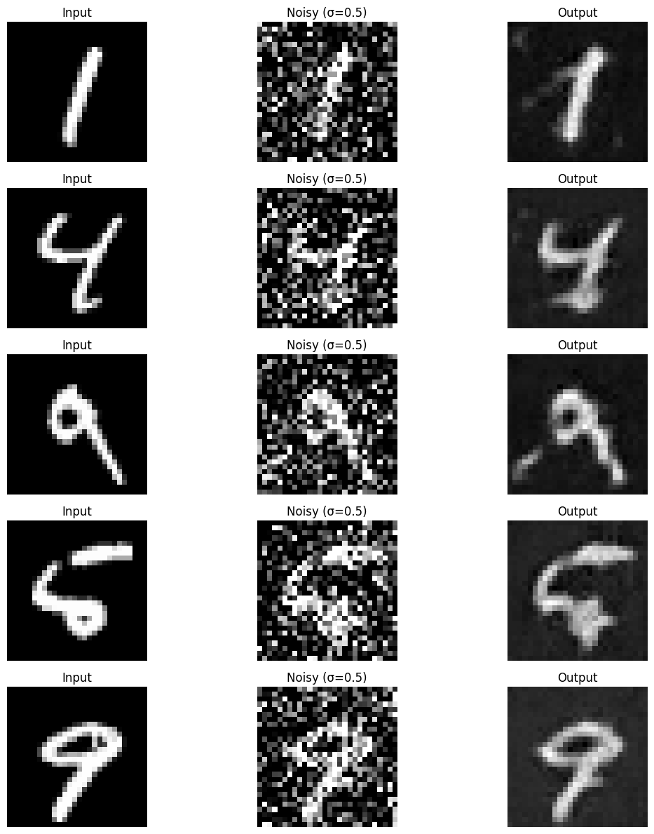
(Original, Noised, Denoised) images after 1 epoch of UNet Training
Below is the results of training over 5 epochs!
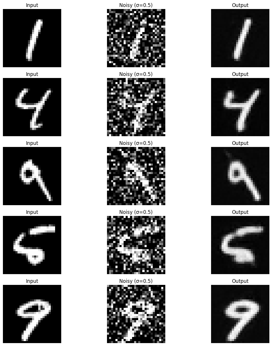
(Original, Noised, Denoised) images after 5 epoch of UNet Training
We see that the model at 5 epochs of training is clearly a bit better at denoising the test image, but the 1 epoch model performs very impressively already.
1.2.2
What if we passed in inputs with noise coefficients that it wasn't trained on? What if we change vary sigma to something it wasn't trained on? This section will explore that
We vary sigma over a diverse range of values between 0.0-1.0 to get the denoising results of our 5 epoch model.
Here are some results:

Out of distribution noised images denoised with 5 epoch of UNet Training

Out of distribution noised images denoised with 5 epoch of UNet Training

Out of distribution noised images denoised with 5 epoch of UNet Training
Pretty good results! We can compare with the results using 1 epoch of UNet Training

Out of distribution noised images denoised with 1 epoch of UNet Training

Out of distribution noised images denoised with 1 epoch of UNet Training

Out of distribution noised images denoised with 1 epoch of UNet Training
We see that it is clear that the 5 epoch model improved significantly from the 1 epoch model in terms of out of distribution noised test set images.
2
Now, we train an actual diffusion model. The difference here is that instead of directly predicting the denoised image, we want to predict the noise that was added to the clean image during the generation of the noised image. We use this actual diffusion model, so we can mimick the iterative denoising process that we saw in Part A, for a simple dataset like MNIST.
Mathematically, our loss function is now a L2 loss on the noise vector, rather than the resulting (clean) image vector, as follows:
Where epsilon_theta is a UNet denoising model(the diffusion model).
Our eventual goal is to be able to sample z from pure noise, rather than just simply a noised MNIST image, and have the denoiser model work well anyway.
2.1
Our training procedure can be described as follows:

Diffusion model constants and training procedure
Our training algorithm can be described as follows:

Algorithm for training Time Conditioned UNet
We add time conditioning to the UNet, making it a time conditioned UNet. We do this through two pairs of a series of linear layers, which we call the FCBlock. This linear FCBlock takes in a constant (t) and outputs a tensor of shape (D, 1, 1) and (2D, 1, 1) respectively, which are added to the block in the UNet after the first Upblock (before concatenation) and also the Unflatten procedure (before concatenation). This is shown in the below diagram:
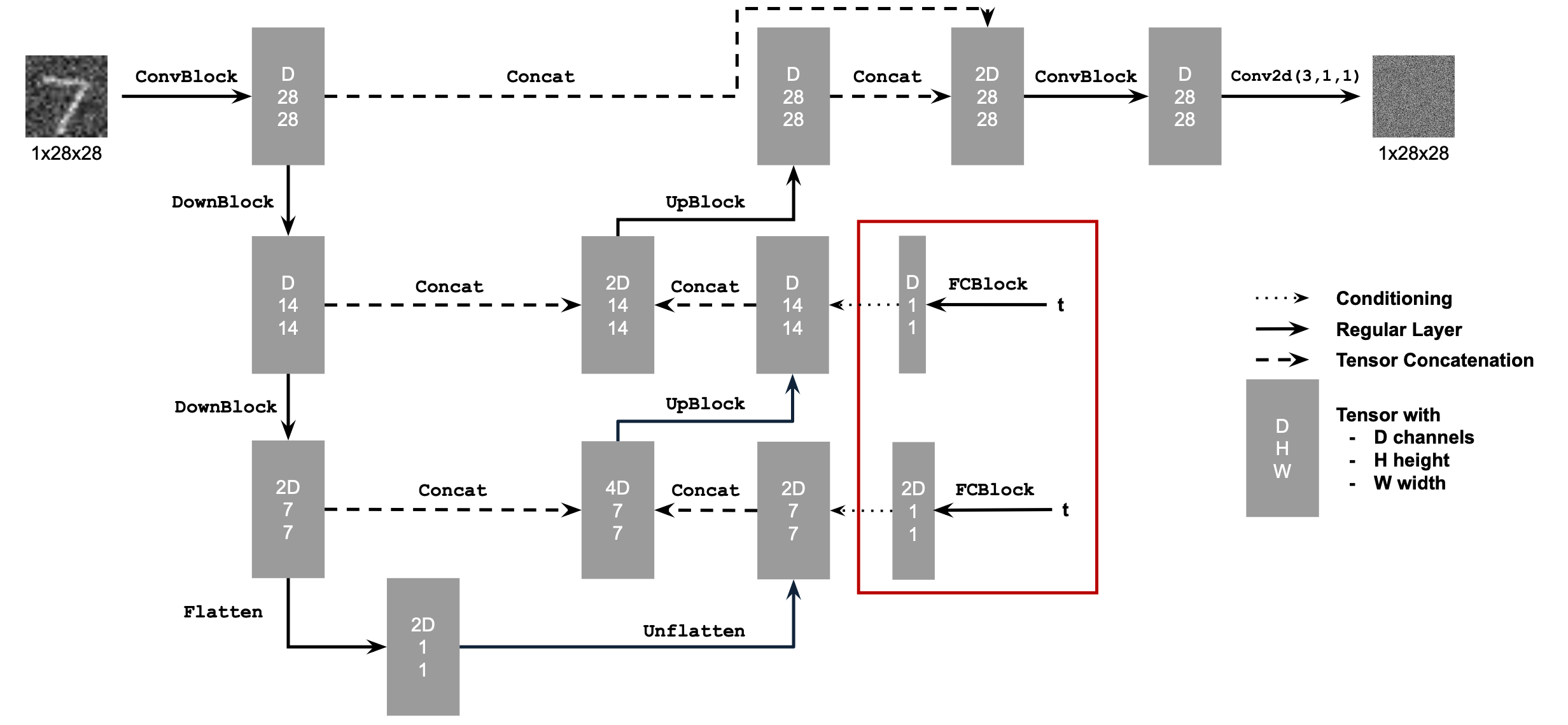
Time Conditioned UNet Structural Diagram
We repeat the training loop for num_epochs=20 epochs, since predicting noise is a more difficult task than denoising. We use a hidden dimension of D=128, and an Adam Optimizer learning rate of 1e-3, with a learning rate scheduler of (0.1)^ (1.0/num_epochs). The scheduler will decrease the learning rate by the factor every epoch. Our batch_size = 128.
2.2
Our (log) training losses per step graph is as follows:
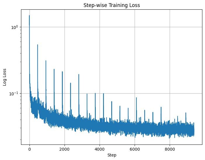
Log Loss over Steps for Time Conditioned UNet
2.3
Now, using our time conditioned model, we can finally sample random noise, and watch as our model (iteratively) transforms the noise into nice images! The algorithm snapshot I followed are as follows:

Time Conditional Algorithm Snapshot
We compare the results for the model trained with 5 epochs and 20 epochs. Here are our sampling results:
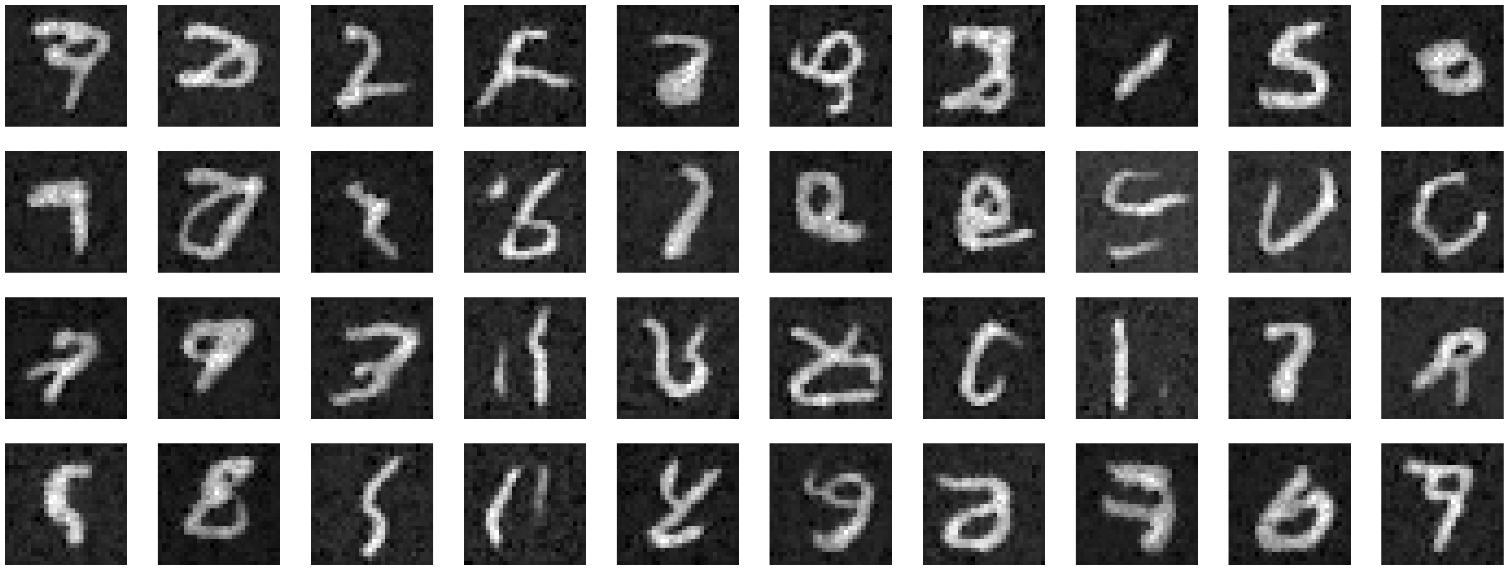
Time Conditional Algorithm Sampling results, 5 epochs
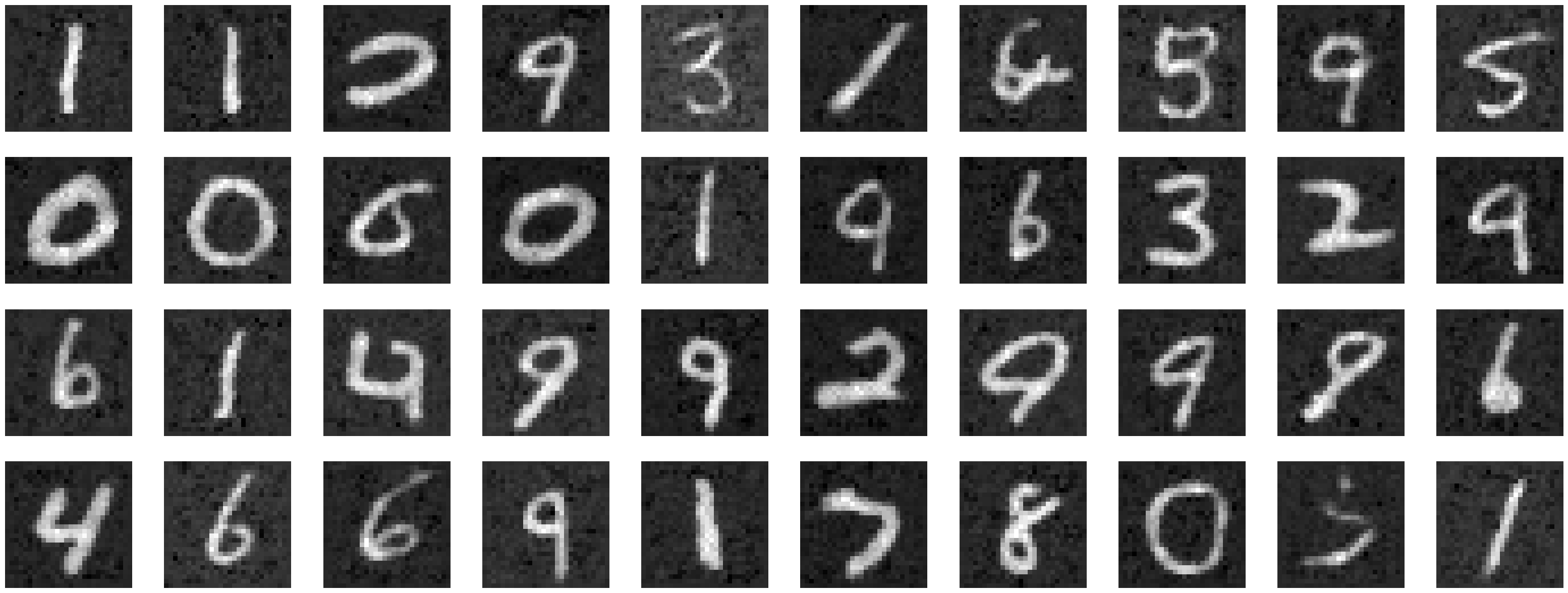
Time Conditional Algorithm Sampling results, 20 epochs
(B&W) Gifs of the interpolation!
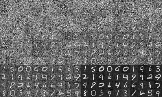
Denoising Gif, 40 images from noise to iteratively denoised image
2.4
Now, we would like to condition the output on the class. We would like to be able to force the model to output class-specific images for random noised input, depending on a class parameter that we pass in.
The way we accomplish this is by adding two more FCBlocks, taking in one hot encoded inputs of shape (N, 10), since 10 is the number of classes of this MNIST dataset. The FCBlocks in this case will output, after executing its linear layers, output tensors of shape (N, D) and (2N, D), where D=hidden_dim. These output tensors will affect the exact same components of the UNet; the result after the first UpBlock as well as the result after the Unflatten Block. The difference, however, is that the output of the FCBlocks here will not be added to the components; it will instead serve as the coefficient of the original blocks, UpBlock and UnFlatten.
We do not want the model to lose the ability to generate images without conditioning, however. My solution is then to pass in a one_hot encoding of all zeroes with a probability of 0.1, forcing the model to learn to also be able to generate quality images even when no class conditioning information is provided.
Training is very similar to time conditioned UNet training, with the exact hyperparameters. The only difference being the addition of the class labels of the MNIST dataset to the training.
Here is the training Algorithm Card:
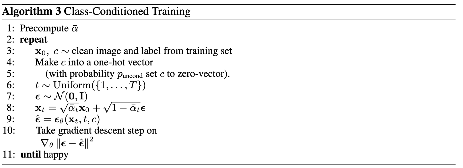
Algorithm for training Time and Class Conditioned UNet
After training, we get the following (Log) loss vs Steps Graph
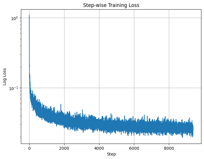
Time and Class Conditioned UNet (Log) loss vs Steps
2.5
Here our sampling procedure is very similar to the way we did it with time conditioned UNet. However, here we use classifier free guidance to get our final value for noise.
With gamma equal to 5, and epsilon_u and epsilon_c being the unconditioned (c=0) and conditioned noises
Like in Part A of the project, we basically extrapolate the noise so that it is further away from the unconditioned noise by 5 times, along the line that connects the conditional and unconditional noise vectors.
Our results for epoch=5 and epoch=20 are as follows:
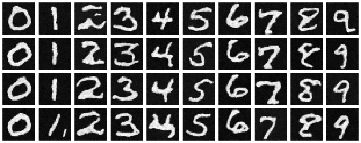
Time and Class Conditioned Sampling with the 5 epoch model
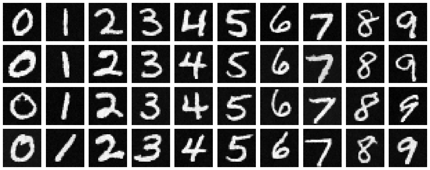
Time and Class Conditioned Sampling with the 20 epoch model
(B&W) Gifs of the interpolation(Using the best, 20 epoch model)!
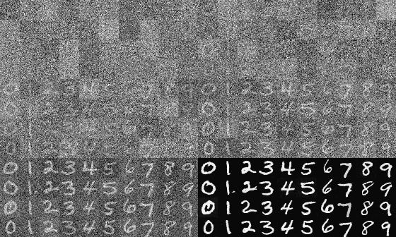
Denoising Gif, 40 images from noise to iteratively denoised image, with class conditioning
Reflection
I really enjoyed this project. In fact, it was probably one of my most favourite projects so far! Free from the pain of having to debug too excessively (unlike Project 3 and 4, trying to align images well was a painstakingly time consuming task), this project was the most fun project for me and I really really enjoyed the cool results it generated.
The project taught me how important iteratively denoising is, and how powerful diffusion models can be when it comes to generating cool images. It also made me realize how difficult a task it is to accurately denoise images. I find the image infilling part to be the most interesting; I did not know that noising the campanile and having it generate high quality images could produce such good, but otherwise seemingly random looking images.